Hey there! It's been a while since I've written a technical blog post. Last month, I came across FP Launchpad, a research center at IIT Madras that aims to build long-term research and educational capacity in the field of functional programming in India. After digging a bit deeper, I came across their kickoff event talks and after watching a couple of them and going through Prof. KC Sivaramakrishnan's blog posts, I kinda got hooked onto functional programming in a way.
I was always kinda curious about functional programming. A couple of my friends used to participate in Advent of Code (AoC), and we would try picking different languages each year. This was one of the ways I learned new programming languages. I remember very well when one of my friends was using Haskell for one of the AoCs, and when I tried to understand his code, it just felt complicated. There were a lot of words - monads, monoid, thunks, bifunctor, etc. This was one of the main reasons I never tried functional programming earlier: the word soup and jargon-heavy terminology.
I took some time out last weekend to try out Not really sure if I can call building an untyped lambda calculus interpreter as "trying" out FP functional programming, but with the lowest number of abstractions. So I decided to build a small untyped lambda calculus interpreter in Go. This blog post would act like an introduction to lambda calculus rather than a "How to build an untyped lambda calculus interpreter" hand-held guide. If you're curious about the untyped lambda calculus interpreter which I made, you can check it out over here.
Firstly, don't get confused by the word "calculus". It is not related to integrals or derivatives in any way. The word calculus just means a formal system of calculation. The part of calculus that deals with integrals and derivatives was mainly developed by Newton and Leibniz, and it became so dominant that people nowadays directly associate calculus with it.
In computer science, there are two major mathematical models of computation - turing machines and lambda calculus. Both are very primitive machines capable of executing any computer algorithm.
In the case of turing machines, it involves an infinite memory tape which is divided into cells that hold a symbol and a pointer that points to one of those cells. At each step, the pointer reads the symbol from the cell, performs some execution based on it, like updating the symbol at the current cell, moving left/right, or halting the machine.
In the case of lambda calculus, all you have are functions. Yep, just using functions and function calls, it is possible to build a universal machine.
Attention Functions are all you need! Specifically higher-order functions
Lambda calculus has three syntactic constructs:
The way you define a function in lambda calculus is as follows:
\[\lambda x.M\]where \(\lambda\) is used to indicate the start of a function which is then followed by a variable (in this case \(x\)) and . (dot) is used as a divider between the function argument and body. It is very similar to how you define annoymous functions in modern-day programming languages. \(\lambda x.x\) is equivalent to lambda x: x in Python.
This is how you execute the functions:
\[(\lambda x.M) \; y = M[x := y]\]The above operation would replace all the mentions of \(x\) in \(M\) with \(y\). This isn't fully true, and I'm gonna cover how the actual function evaluation takes place in depth in the substitutions section.
Even though both turing machines and lambda calculus refer to the same thing, i.e., a universal machine, both of them are adopted by different communities within the field of computer science research. The design of turing machines is much more low-level/bare bones, and hence it is used by researchers working on computer algorithms, whereas lambda calculus is used by programming language researchers. Lambda calculus focuses more on the structure of your program, i.e., how you organize your program.
Lambda calculus is the most minimal turing complete language as it just consists of three different production states. Here is the entire BNF grammar of lambda calculus:
Semantically, it consists of majorly two things - \(\alpha\)-conversion and \(\beta\)-reduction. Before jumping into them, I would like to go over a couple of other topics, as they are utilized to formally define the aforementioned semantic rules. There is something called \(\eta\)-conversion as well but it is often omitted.
In lambda calculus, a variable is either bound or free depending on whether it appears within the scope of a corresponding \(\lambda\). A \(\lambda x\) term introduces \(x\) into the scope immediately after the dot, and \(x\) remains in the scope until the end of the term that \(\lambda x\) governs, which is determined by the parentheses.
For example, in \(\lambda x.\lambda y.xy\), \(x\) comes into scope after the first dot and spans throughout the entire body, whereas \(y\) only comes into scope after the second dot. The lifetime of each of the local variables can be visually understood through the parentheses around their corresponding \(\lambda\) terms.
\[ (\lambda x.(\lambda y.xy)) \]In the lambda expression \(\lambda x.xy\), \(x\) is said to be bound variable because it was brought into scope right after the first dot whereas \(y\) is said to be free variable because there is no corresponding \(\lambda y\) term in the expression via which \(y\) would have been brought into scope.
In the lambda expression \((\lambda x.x) (\lambda y.yx)\), \(x\) is both a bound and free variable
\[ (\lambda x.x) (\lambda y.yx) \]Over here, the first \(x\) is brought into scope after the first dot, i.e., right after \(\lambda x\), and it goes out of scope when it encounters the first closing parentheses. In the second lambda term, only \(y\) was brought into scope, due to which the second \(x\) is a free variable, whereas \(y\) is a bound variable.
Formally, the set of free variables for a lambda term \(t\) is written as \(FV(t)\) and is defined as:
Substitution is a mechanism by which free occurrences of a variable are replaced with another lambda term. it is generally represented as \(M[x := N]\), which means “replace all the free occurrences of \(x\) in \(M\) with another lambda term \(N\)”. It is very important to note that replacing of variables via substitution is only done for free variables, because replacing bounded variables completely alters the meaning of the lambda function.
If \(x := y\) substitution rule was applied on \(\lambda x.x\) which is then identity function then it changes into a constant function:
\[ \lambda x.x[x := y] = \lambda x.y \]If you see the identity function has been changed into a constant function, i.e., the lambda function's meaning has been completely changed.
Apart from the above issue, there could be another problem that might arise during substitution, which is often referred to as “variable capture”. Consider the following example
If \(y := x\) substitution rule is applied on \(\lambda x.y\):
\[ \lambda x.y[y := x] = \lambda x.x \]In the above reduction, we replaced all the free occurrences of variable \(y\) in the lambda function with \(x\), but still, it changed the meaning of the function. The reason behind this is that the binder \(x\) and the \(x\) with which we have to replace both of them need to be treated differently. Over here, the free variable \(x\) gets captured by the binder \(x\).
One way to resolve this issue is via using a technique called \(\alpha\)-renaming, where the bound variables of a lambda function are renamed in a consistent manner such that the meaning is quite preserved i.e. \(\lambda x.x\), \(\lambda y.y\) and \(\lambda z.z\) all refer to the exact same function even though the binders have different names.
So, considering a bit more generalized version of the above example: \((\lambda x.y)[y := N]\). Over here, first it needs to be checked whether \(x\) belongs to the set of free variables of \(N\). If yes, then \(\alpha\)-rename must be done. The binder \(x\) needs to be renamed into a different binder \(z\) such that \(z \notin FV(N)\).
\[ \lambda x.y[y := x] = \lambda z.y[y := x] = \lambda z.x \]Mathematically, substitution can be defined as follows:
It might be a bit difficult to grasp the core intuition directly from the above mathematical expressions. Here is a breakdown of each case:
In the previous section, I have covered a bit about \(\alpha\)-renaming. Within this section, we'll try to properly get an intuition of what \(\alpha\)-conversion is. It is one of the two major semantic rules within lambda calculus.
\(\alpha\)-conversion is a mechanism to rename the bound variables of a lambda function consistently such that its meaning is preserved, i.e., \(\lambda x.x\), \(\lambda y.y\), and \(\lambda z.z\) all refer to the same function even though their binder variable have different names. Two lambda terms are said to be \(\alpha\)-equivalent if one can be transformed into the other via some finite series of \(\alpha\)-conversions.
\(\lambda x.M\) and \(\lambda y.M[x := y]\) are said to be \(\alpha\)-equivalent, if \(y \notin FV(M)\). \(\alpha\)-equivalence between two lambda terms is commonly represented as \(\lambda x.M \equiv_{\alpha} \lambda y.M[x := y]\).
\(\beta\)-reduction is all about how to evaluate the applications. As lambda calculus consists of variables, functions, and function calls, the only way a program can be built is via executing the functions, i.e., layers of applications. An application is generally represented as \((\lambda x.M) N\) and an unapplied application is often referred to as “redex”. The way \((\lambda x.M) N\) is evaluated is using substitutions:
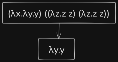
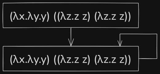
\[ (\lambda x.M) N = M[x := N] \]While applying \(\beta\)-reduction to a lambda function, one would come across different forms of a lambda term, and all of them mathematically have the same meaning. \((\lambda x.(\lambda y.y) x) z\) and \(z\) both are mathematically equivalent to one another, but the former is an intermediate form (i.e., it can be reduced further down), whereas the latter is in its most simplified form, and it can't be reduced down further. A lambda term that can't be further reduced is said to be in “normal form”. It is important to note that not all terms have a normal form. For example, \((\lambda x.x \; x) (\lambda x.x \; x)\) can't be reduced down to a normal form, as on reduction you keep getting itself, it is equivalent to calling a function within itself.
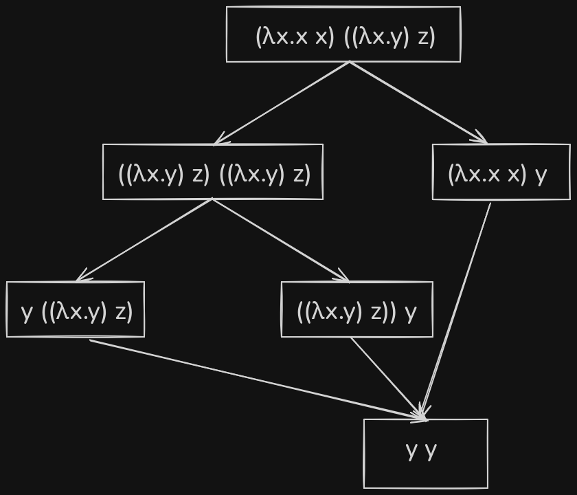
Let's take an example lambda expression and try to evaluate it - \((\lambda x.x \; x) ((\lambda x.y) z)\)
The above reduction graph shows all the possible ways to reduce the example lambda expression down to its normal form. There are different styles of evaluation used. In the right branch of the reduction graph, the inner redex is first evaluated, as compared to evaluating the outer redex in the left branch. Over here, it didn't matter which path was chosen as all of them led to the same answer, but there are cases where, depending on the evaluation method, the result changes.
Consider another example lambda expression - \((\lambda x.y) ((\lambda x.x x)(\lambda x.x x))\)
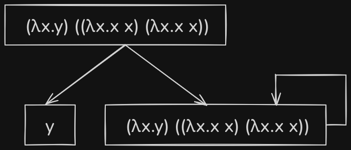
Over here, if the outer redex was evaluated first, then \(y\) would be the output, as there are no free occurrences of \(x\) in \(y\) for substitution to occur. But if the inner redex was chosen to be evaluated first, then it gets stuck in this recursive loop.
If you notice, the naïve \(\beta\)-reduction (aka \(\beta\)-reduction) is very non-deterministic. To make it a bit clearer, here is how \(\beta\)-reduction can be described formally using inference rules:
The way an inference rule \(\frac{P}{Q}\) is read is "if \(P\) is true then \(Q\) happens". Over here, \(P\) is said to be the premise and \(Q\) is said to be the conclusion. Keeping that in mind, let's now go through each of the above inference rules and understand them in a simpler language, going from top left to right.
The goal of full-\(\beta\) reduction is "if there is a redex, then reduce it down". There is no hierarchical structure in terms of the reduction order. Due to this nature of full-\(\beta\) reduction, the non-determinism arises, which can be clearly seen in example 2.
Until now, we have only checked at full-\(\beta\) reduction which is a non-deterministic reduction strategy. There are other reduction strategy which attempts to fix the issues with full-\(\beta\) reduction. For the scope of this blog, we would mainly focus on the following reduction strategies:
The core idea of normal order is to reduce the leftmost, outermost redex first. The most important property of normal order is that if a term has a normal form, then normal order reduction will find it. This is what the "Church-Rosser" theorem is all about. I wouldn't be going too deep into that theorem within this blog, but if you are interested in reading more about it, I would suggest reading this paper titled "Church–Rosser Made Easy".
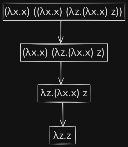
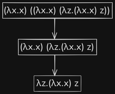
To get a better intuition of normal order, let's try to evaluate a lambda expression using it - \((\lambda x.x) ((\lambda x.x) (\lambda z.(\lambda x.x) z))\).
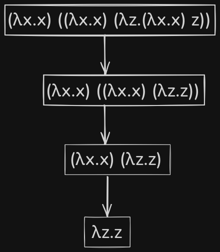
Here is the \(\beta\)-reduction of the same lambda expression but using full-\(\beta\) reduction. Over here, the innermost redex is reduced first.
Let's take another example where full-\(\beta\) reduction fails due to its nature of evaluating the innermost redexes first.
In the above example, consider the recursive lambda term \((\lambda z.z \; z) (\lambda z.z \; z)\) as \(\Omega\).In case of normal order, it evaluated the outermost redex right and as there were no free \(x\) in \(\lambda y.y\), the evaluated output was \(\lambda y.y\). In case of full-\(\beta\) reduction, the inner redex was attempted to be evaluated first, and as the inner redex was a recursive lambda term, the evaluation got stuck in a loop.
Call-by-name reduction strategy is very much similar to normal order, except for one part, i.e., it doesn't reduce within lambda bodies. In last step of example 3, the body of \(\lambda z.(\lambda x.x) z\) was reduced to finally get \(\lambda z.z\). The functionality of reducing a lambda's bodies without an application might feel unintuitive, as in regular programming languages, a function's body is evaluated only when it is executed. To avoid this confusion, call-by-name reduction strategy is used, which is exactly like normal order, except it doesn't allow reduction within lambda bodies.
In call-by-name, the function arguments are passed unevaluated and only reduced if they end up in a function position, i.e., the left-hand side of an application. This avoids evaluating arguments that are never used. However, if an argument is used multiple times, then call-by-name re-evaluates it each time. Call-by-need solves this issue using a cache mechanism. Call-by-need memoizes the result of the first evaluation, and it is reused in other places; due to this mechanism, any argument is reduced at most once. This is also known as “lazy-evaluation," and it is exactly what Thunk in Haskell means.
Call-by-value is kind of like on the other end of the spectrum, while comparing it to call-by-name and call-by-need. In call-by-value, before applying a function, the arguments are fully evaluated first, and then proceed forward with the substitution. The benefits of call-by-value over call-by-name (or call-by-need) are that it's predictable and cheap per step, as all the arguments are fully evaluated before the function is executed. The cons of it are:
Until now, we have seen how functions can be evaluated using \(\beta\)-reduction and how two functions are equivalent to each other using \(\alpha\)-conversion. Lambda calculus by itself doesn't have any data structures, i.e., there are no booleans, numbers, floats, lists, tuples, etc. It only has functions. To mimic the behaviour of actual data structures in lambda calculus, church encodings are used. The list of all possible encodings is very huge, so instead of this blog, we'll mainly blog on the church encodings of booleans, numbers, logical operators (AND, OR, NOT), arithmetic operators (successor, addition, and multiplication), and pairs. I've tried to restrict the number of encodings so that the blog doesn't end up being about church encodings rather than being a primer about untyped lambda calculus.
The way true is defined in lambda calculus is that it is a function that takes in two arguments and returns the first one, whereas false is a function that also takes in two arguments and returns the second one.
Using the above definitions of booleans, we can structure a function which mimics the behaviour of if/else branch as follows:
Over here, the first argument is the "boolean function", the second argument is equivalent to the if branch, and the third argument is equivalent to the else branch. So, if the boolean function is true then it'll return the first option, i.e., the if branch will be executed and vice versa.
After understanding how boolean church encoding works, the encoding for logical operators would look much more intuitive. Let's try to walk through the process of creating an encoding for the AND logical operator.
The signature of the AND function would take in two arguments, which would be boolean functions and return a boolean function as output. Let's take a look at the truth table of the AND gate.
| A (Input) | B (Input) | Y (Output = A & B) |
|---|---|---|
| F | F | F |
| F | T | F |
| T | F | F |
| T | T | T |
Now treating the above truth table as a function input/output table, we can see that the output of the function is always F if either one of them is F and if either one of them is T then output is equal to the value of other argument.
Similarly for OR operator, we'll first analyze the truth table as a function input/output table and understand the patterns.
| A (Input) | B (Input) | Y (Output = A | B) |
|---|---|---|
| F | F | F |
| F | T | T |
| T | F | T |
| T | T | T |
Over here, we can see that if either one of the arguments is T then the output is T and if either one of them is F then the output is equal to the value of the other argument.
And finally for NOT operator
| A (Input) | Y (Output = !A) |
|---|---|
| F | T |
| T | F |
In the case of NOT function, it would only take in a single argument. If the argument is T then return F and if it is F then return T.
The way numbers are defined in church encoding is very interesting. A number is defined as a function that takes in two arguments - \(x\), which is a starting point for all the numbers, and \(f\), which is a function that returns the successor of any number.
The definition of a number and the successor function in church encoding are kind of intertwined with each other. Let's try to get a better intuitive understanding by trying to evaluate succ one:
If you've ever used partial functions in Python (functools.partial) then that's exactly what we've done with succ one. succ function in total takes in three arguments, but we've passed one of them, and it generated a partial function out of it.
If you wanted to perform 1 + 2 in lambda calculus, it would be equivalent to replacing the "starting point" (\(x\)) in 1 with 2
So performing \(m\) + \(n\) is equivalent to equivalent \(x\) in \(m\) with \(n \; f \; x\)
\[ \text{Add} = \lambda m.\lambda n.\lambda f.\lambda x.m \; f\; (n \; f \; x) \]If you wanted to perform 2 * 3 in lambda calculus
So in case of multiplication, rather than replacing the "starting point", you replace the successor function (\(f\)) with \(n \; f\) in case of \(m \times n\). The idea is very similar to how multiplication is basically repeated addition.
\[ \text{Mult} = \lambda m.\lambda n.\lambda f.\lambda x.m \; (n \; f) \; x \]Pairs are basically equivalent to a tuple with two elements in this case, and the way this can be thought of in the context of functions is that it is a function that takes in two arguments, which correspond to the first and second elements of the pair.
\[ \text{ConstructPair} = \lambda m.\lambda n.\lambda b.b \; m \; n \]When both of the elements are passed, the constructor returns a partial function \(\lambda b.b \; m \; n\). This partial function is later used by the accessor functions to retrieve the individual elements.
\[ \begin{aligned} \text{First} &= \lambda p.p \; \text{True} \\ \text{Second} &= \lambda p.p \; \text{False} \end{aligned} \]Here's a small demo of my untyped lambda calculus interpreter computing \(\text{fib}(n=3)\) (3rd term in fibonacci sequence) which is 2 (or) \(\lambda f.\lambda x.f \; f \; x\) in church encoding. Over here = is an assignment operator for defining macros, which are just short snippets of reusable lambda expressions.
true = \a.\b.a
false = \a.\b.b
zero = \f.\x.x
succ = \n.\f.\x.f (n f x)

is_zero = \n.n (\x.false) true
plus = \m.\n.\f.\x.m f (n f x)
pred = \n.\f.\x.n (\g.\h.h (g f)) (\u.x) (\u.u)

yy = \f.(\x.f (x x)) (\x.f (x x))

fib = yy (\f.\n.(is_zero n) zero ((is_zero (pred n)) (succ zero) (plus (f (pred n)) (f (pred (pred n))))))
fib (succ (succ (succ zero)))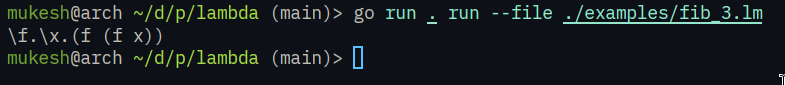
Phew! This ended up being a bit too long, but I have enjoyed every single part while researching and studying about lambda calculus, and also while building the interpreter for it. It was such a fun rabbit hole, especially the church encoding part, it sorta introducted me to this new methodology on how to think about writing programs.